Figure Captions
|
|
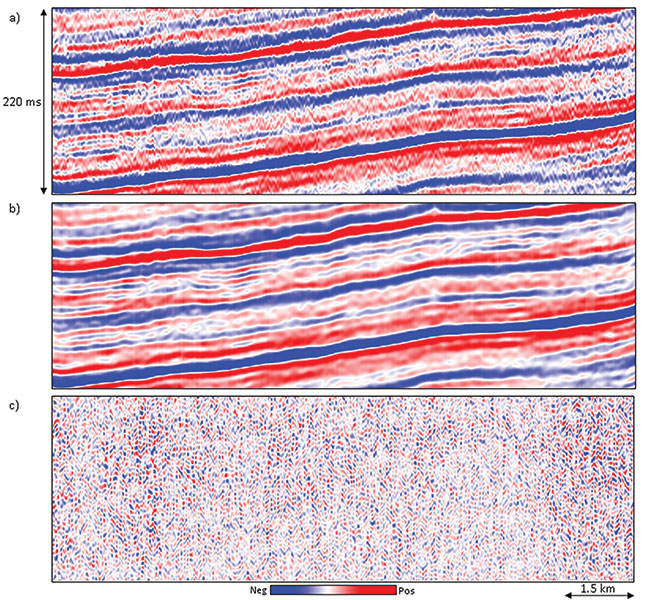
Figure 1. Vertical slice through  seismic seismic amplitude volumes (a) before, and (b) after principal component structure-oriented filtering, and (c) the difference section. Notice the broken inclined wave trains of noise are seen in the difference section and the display after structure-oriented filtering looks clean with the reflections much more coherent. (Data courtesy of Arcis Seismic Solutions, TGS) amplitude volumes (a) before, and (b) after principal component structure-oriented filtering, and (c) the difference section. Notice the broken inclined wave trains of noise are seen in the difference section and the display after structure-oriented filtering looks clean with the reflections much more coherent. (Data courtesy of Arcis Seismic Solutions, TGS) |
|
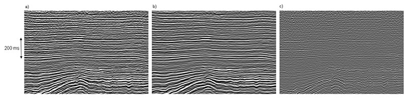 |
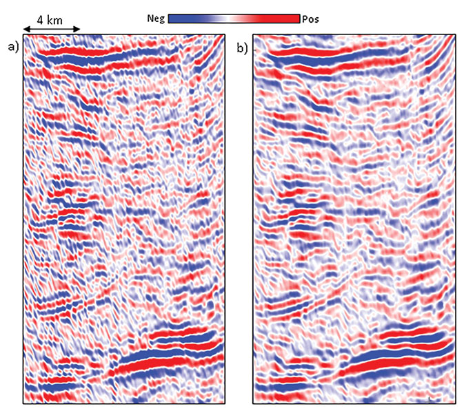
Figure 2. Vertical slices through legacy data acquired over Vacuum Field, New Mexico (a) before, and (b) after edge-preserving structure-oriented filtering using the default parameters in a commercial software implementation. (c) The difference between the two, showing the desired rejection of the steeply dipping migration artifacts, but also of the higher frequency components of the seismic signal. (Data courtesy of Marathon Oil Co.) |
|
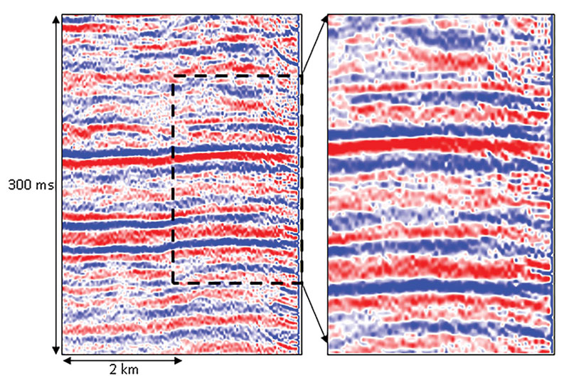 |
Figure 3. Segment of an inline seismic section very close to the edge of the survey. Notice the edge effect to the right (migration smiles), as well as the noise in the data. A zoom of the portion in the dashed rectangle shows the noise bursts and the incoherency of the reflections. (Data courtesy of Arcis Seismic Solutions, TGS) |
|
|
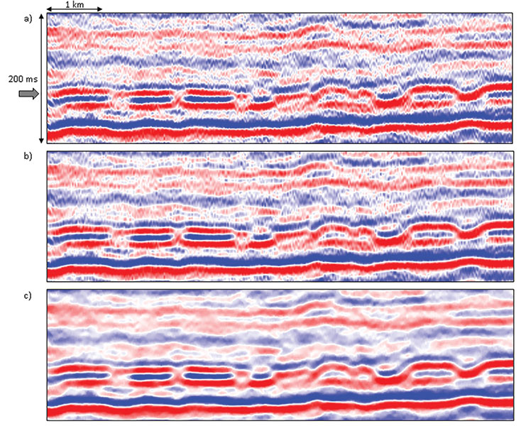
Figure 4. Segment of a seismic section from (a) the input seismic volume, (b) the same data after structure-oriented filtering, and (c) the same input data after 3-point median filtering. Notice the fine amplitude bursts are taken care of much better with median filtering than structure-oriented filtering. (Data courtesy of Arcis Seismic Solutions, TGS) |
|
|
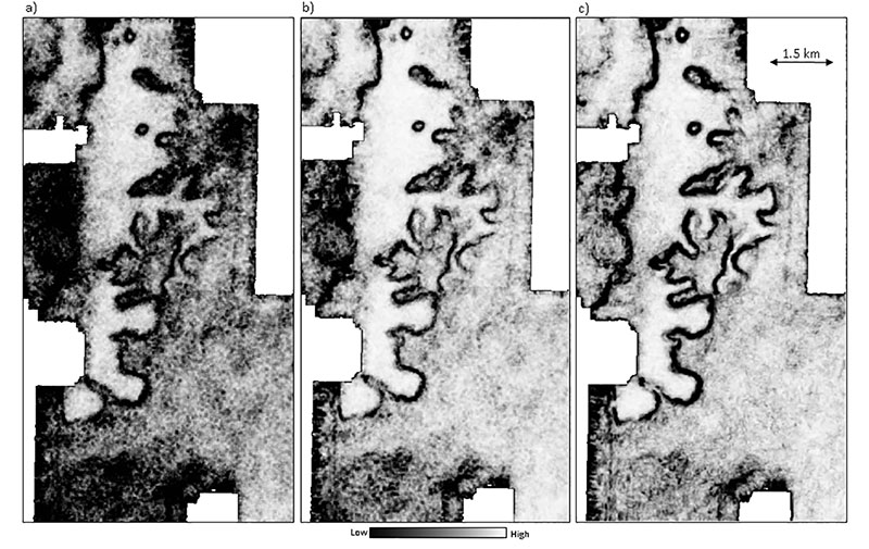
Figure 5. Time slices (at 1362 ms) from the coherence volume generated on (a) input seismic data volume, (b) input seismic data volume with structure-oriented filtering, and (c) the input with median filter. Notice the clarity on the coherence run on median filtered output as compared with coherence run on input data with structure-oriented filtering. (Data courtesy of Arcis Seismic Solutions, TGS) |
|
|
Figure 6. Segment of a seismic section from (a) the input seismic volume, and (b) the same data after filtering coherent noise using a dip filter. Notice the dipping noise has been suppressed and the reflections are looking more coherent and continuous. (Data courtesy of E&B Resources) |
|
|
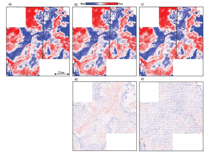
Figure 7. Time slice at t=1044 ms through seismic amplitude volumes (a) before, (b) after principal component structure-oriented filtering, and (c) after 3-point median filtering. Notice the background noise is better suppressed by the median filtering than by the principal component structure-oriented filter. However, while the E-W acquisition pattern seen seems to be toned down a bit after filtering, it is not eliminated completely. The black dashed line shows the location of the crossline segments. The difference displays between (a) and (b) and (a) and (c) are shown in (d) and (e) respectively. (Data courtesy of Arcis Seismic Solutions, TGS) |
|
|
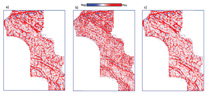
Figure 8. Time slices through most-positive curvature volumes generated at (a) long-wavelength, (b) intermediate wavelength, and (c) long-wavelength after foot-print filtering. Notice the north-south footprint pattern has been suppressed after kx-ky filtering of the input data. (Data courtesy of Arcis Seismic Solutions, TGS) |
|
|
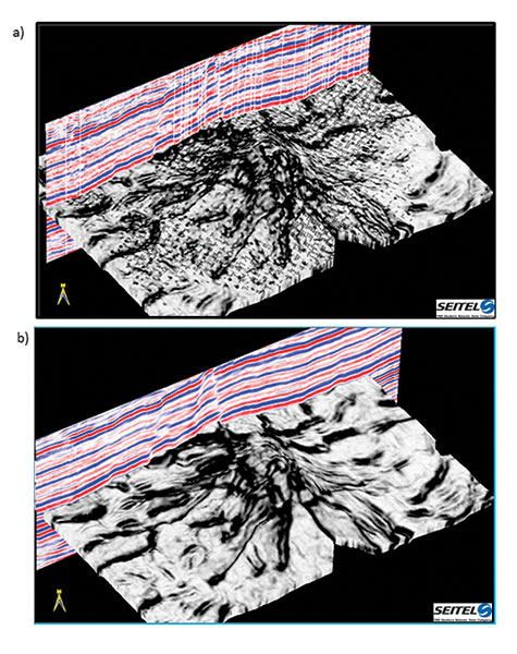
Figure 9. Chair displays with the vertical as seismic and the horizontal as stratal slices from the coherence volumes (a) before, and (b) after 5-D interpolation. The missing traces in the seismic have been predicted and the coherency of the reflections looks much better. The coherence attribute generated from the interpolated data also looks much better. (Data courtesy of Seitel Data) |
|
|
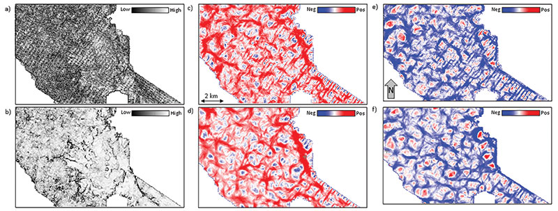
Figure 10. Time slices at 158 ms through coherence volumes (a and b), most-positive curvature (c and d), and most-negative curvature (e and f) computed from amplitude data (above) before, and (below) after 5-D interpolation. Notice the acquisition footprint has been suppressed after 5-D interpolation. (Data courtesy of Arcis Seismic Solutions, TGS) |
Suppression of Noise
Of all the types of noise, random noise – or coherent noise that appears random – is the easiest to suppress. The mean filter is the simplest and most familiar noise suppression filter. These filters simply represent the arithmetic running average of a given number of spatial samples, usually "3" for 2-D data or "5" for 3-D. Larger filters are most efficiently implemented by cascading, or reapplying, the filter to a previously filtered version of the data multiple times. Mean filters can be directly applied to time structure maps and horizon slices through seismic amplitude or attribute volumes. In 3-D, mean filters should be applied along structure rather than along time slices, generating a "structure-oriented" filter. In general, mean filters centered about the trace to be filtered will smear lateral discontinuities in the seismic data, and should be avoided.
In contrast, a structure-oriented median filter not only suppresses random noise, but will preserve lateral reflector discontinuities. The median filter picks up samples within the chosen aperture along the local dip and azimuth and replaces the amplitude of the central sample position with the median value of the amplitudes. Principal component filters go one step further by using more than the five (or more) samples along structure dip and azimuth, but also a suite of 2K parallel five-sample slices above and below the target sample.
Mathematically, the principal component generates a five-sample pattern that best represents the lateral variation in amplitude along the 2K+1 slices. In the absence of high amplitude artifacts in the data in general, the principal component filter accurately preserves lateral changes in seismic amplitude and rejects noise. All of these filters can be run in an edge-preserving manner.
The simplest way to preserve edges is to simply compute the location of the edges using a coherence or Sobel filter algorithm sensitive to discontinuities. The desired filter is then applied only to those areas where the coherence falls above some user-defined value. A slightly more complicated way to preserve edges is to evaluate the standard deviation (or alternatively, the coherence) in a suite of overlapping windows that include the analysis point. Then the mean, median, principal component or other filter is computed in the window with the smallest standard deviation or coherence and mapped to the desired sample.
Examples
We show the application of a principal component structure-oriented filtering to a data volume through a representative seismic section in Figure 1. The input data in Figure 1a shows good reflectors with subtle cross-cutting noise. The filtered section (Figure 1b) exhibits improved event continuity and preserved amplitude. To ensure that no useful reflection detail is lost in the filtering process, we take the difference volume and examine it.
As seen in Figure 1c, there are no reflection events that have been rejected. Instead, we see random noise as well as inclined broken noise patterns. This steeply dipping noise is common to most seismic data volumes and is associated with the migration of shallow reflections, diffractions and coherent noise that have been insufficiently sampled, or aliased, in the spatial acquisition design.
Modern "high density" acquisition directly addresses these sampling problems and results in superior images for the interpreter. Structure-oriented filtering is widely used in the industry and has also found its way into most commercial workstation interpretation software packages. It usually works fine in most cases, and so the interpreters tend to use it all the time, irrespective of the quality of the input seismic data. We wish to elaborate on this aspect and emphasize that suppression of noise should be done carefully, only after examining the quality of the data. Parameters can be important. In general, one should avoid running filters vertically, since this will result in lower frequency output (Figure 2).
In this example, the edge-preserving, structure-oriented filtering was run with the default parameters in a popular commercial seismic interpretation package. These default parameters result in smoothing not only along dip, but also perpendicular to dip, thereby acting as a low pass filter. One should always examine the rejected noise by computing the difference between the input and output as shown in Figure 1c and Figure 2c.
In Figure 3a, we show a small segment of a seismic section close to the edge of the survey. The data at the edge of the survey to the right side of the display has migration smiles. Seismic migration takes each sample of the input data and maps it to a 3-D ellipsoid in the output data. If the sampling of the surface data is sufficiently dense, these smiles constructively interfere along reflectors and diffractors and destructively interfere elsewhere, thereby forming the migrated image.
If the surface data are coarsely sampled, the steeper limbs of the smiles fail to destructively interfere resulting in the steeply dipping artifacts seen in Figure 1 and Figure 2. If the data goes abruptly to zero, such as at the edge of a survey or in a no-permit zone, there are no additional smiles to destructively interfere, leaving the edge effects seen in Figure 3.
High amplitude spikes present in the data also generate smiles, which appear as a number of small amplitude bursts scattered throughout the section in a random way. This is clearly seen on the zoom of a small portion of the section shown in Figure 3b. When such amplitude bursts, or spikes are randomly present in the data, principal component structure-oriented filtering may not be the best way to enhance S/N ratio. In Figure 4a we show a segment of a section from seismic data that has a significant distribution of high amplitude noise bursts distributed in a random manner. The principal component structure-oriented filter application is shown in Figure 4b. Notice the amplitude bursts have been toned down somewhat after the filter application, but have not been entirely suppressed. A similar application of median filtering to the same data shown in Figure 4c demonstrates the complete suppression of the noise bursts. By construction, the principal component filter generates a spatial pattern that best represents the energy within suite of 2K+1 vertical windows.
In the extreme case where one of the traces is a high amplitude spike, the most energetic pattern will be the value 1.0 at the spike trace location and zero at the other locations. Counterintuitively, the principal component filter in this case will preserve the noise and reject the signal. The data in Figure 4 are not quite this bad, but have sufficiently high amplitude noise that it contaminates the pattern.
In contrast, the non-linear median filter is constructed to reject anomalously strong negative and positive spikes, resulting in the improved image in Figure 4c. The coherence attribute using energy ratio algorithm was computed from the input and the two filtered outputs in Figure 4, and their comparison is shown in Figure 5. Notice the sharp definition of the features see on the slices after median filtering as compared with the other two.
Dipping Noise
Steeply dipping noise, sometimes due to shallow backscattered ground roll can also riddle seismic data. If left in the data, this noise will create artificial patterns on the computed attributes. This noise can be suppressed with dip filters. In Figure 6 we show the input and the dip-filtered result. While the filtered result looks cleaner and reflections look continuous, there is always the danger of removing signal by filtering and it should be checked by computing the difference volumes.
Acquisition Footprint
Acquisition footprint refers to linear spatial grid patterns seen on 3-D seismic time slices. Commonly seen on shallower time slices or horizon amplitude maps as striations, they can mask the actual amplitude variations under consideration for stratigraphic interpretation, AVO analysis and reservoir attribute studies.
In land data, acquisition footprint often results in seismic data when the offset and azimuth distribution varies from CMP bin to CMP bin. In marine data, repeatable variations in offset and azimuths often occur due to cable feathering. Spatially periodic changes in offset and azimuth give rise to spatially periodic variations in the stacked data, sometimes from AVO and AVAz effects, but more often from subtle errors in velocities that result in a different stack array response. If the pattern is vertically consistent, and has a similar wavelet to neighboring traces, principal component structure-oriented filtering will consider this consistent amplitude pattern to be signal, not noise, and preserve it.
In Figure 7 we show the application of both principal component and median filters on seismic data, which has an east-west acquisition pattern. Both the filters tend to reduce the effect somewhat, but do not suppress it entirely. The different slices confirm this.
One way to suppress the footprint is to first analyze the pattern in the kx-ky wavenumber domain, and then design filters to remove the unwanted patterns. Of course, one runs the risk of also removing the authentic signatures of fractures in the data that have the same orientation as the footprint, and so such filtering needs to be applied with care. We show one such application in Figure 8, where the most-positive curvature time slices are shown from the input seismic data at a long-wavelength computation (Figure 8a) and at an intermediate wavelength computation (Figure 8b). Both these displays show the north-south oriented acquisition footprint patterns.
The equivalent display from the most positive curvature (long-wavelength) computed on the footprint-filtered version of the seismic data is shown in Figure 8c. Notice the absence of the north-south footprint striations.
Regularization of Seismic Data with 5-D Interpolation
Seismic attributes computed from sub-optimally sampled seismic data or data with missing traces give rise to artifacts. The ideal way to have optimally sampled seismic data is to have an optimal shooting geometry followed through in the field. Practical considerations, however, usually yield seismic data that have missing traces, large data gaps or a non-uniform distribution of offsets and azimuths in the bins. In principle, one might correct for or fill in the missing data gaps by reshooting the data in those areas. In practice, such infill acquisition can be extremely expensive, and is avoided.
The second best approach is to handle the missing data problem in the processing center. Originally, single or a local few missing data traces can be handled by copying adjacent traces to into the CMP bin. Such simplistic methods were superseded by 2-D and later 3-D triangular trace interpolation methods.
All these methods use the local data to predict the missing data and so are called local methods. They do have a limitation in that they cannot handle large data gaps. In the last decade or so, global methods for data interpolation have evolved that use more of the available data to populate the missing data. These methods are multidimensional instead of one-, two- or three-dimensional, operating simultaneously in as many as five different spatial dimensions (e.g. inline, crossline, offset, azimuth and frequency), and are able to predict the missing data with more accurate amplitude and phase behavior.
As might be expected, these methods are compute intensive and have longer runtimes than the local methods. Such 5-D interpolation methods regularize the offset and azimuth distribution in bins, and hence the simulated acquisition geometry of the seismic data. In doing so they address the root cause of the missing data, and subsequent footprint artifacts. In Figure 9 we show chair displays with seismic amplitude as the vertical sections and coherence as the horizontal sections, before and after 5-D interpolation. Notice the missing traces in the seismic before 5-D interpolation are all predicted nicely and the reflections looks more coherent.
Similarly, the speckled pattern corresponding to the missing traces on the coherence volume before 5-D interpolation is gone, and the coherence display is amenable to much better interpretation after 5-D interpolation.
In Figure 10a we show time slices at t=158 ms, where the acquisition footprint appears prominently on the coherence attribute as striations in the NE-SW direction, masking the reflection detail behind them. Figure 10b shows the equivalent coherence slice after 5-D regularization, exhibiting considerable improvement in data quality. Similarly, cleaner and clearer curvature displays are derived from data after 5-D interpolation and resulting in more confident interpretation, as shown in Figure 10c to 10f.
Conclusions
Seismic data usually suffer from different types of noise. Random noise is the easiest to recognize and the easiest to address. Coherent noise such as acquisition footprint can be more challenging and result in coherent artifacts on seismic attribute displays that can mask features of interpretation interest. We have emphasized the importance of conditioning the data in terms of noise filtering as well as regularizing the data with 5-D interpolation. We have suggested that the input data should first be examined carefully to understand the type of noise contaminating them, and then choosing an appropriate method of filtering.
Random noise may be handled using principal component structure-oriented filters, but when spikes or sharp amplitude bursts are present, they could be handled better with nonlinear structure-oriented median filters.
Inclined coherent noise can be handled with dip filtering. Acquisition footprint or missing data issues arising out of non-uniformity in the geometry of the seismic data could be handled with 5-D interpolation. Once such problems are diagnosed and handled for the input seismic data, seismic attributes computed on them would definitely be more meaningful, would display better and thus lead to more accurate interpretations.
Return
to top.